
Logistic regression is one of the most important machine learning algorithms. This post will show you how it works and how to implement it in code using Python.
This post assumes you are already aware of how linear regression works with gradient descent. If not, take a look at this post where I explain linear regression.
Basics of logistic regression
Logistic regression is a classification algorithm that outputs the probability that an example falls into a certain category.
So, if we have a dataset with a single feature and two output categories, 0 or 1, such as that shown by the diagram below:
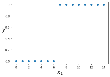
We will be able to fit a curve to the data such as in the diagram below.
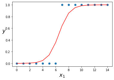
When we have an unseen datapoint that we want to classify, we will look to see where that point falls on the curve. If the curve has a value above 0.5 we will classify the datapoint as a 1, if it is below 0.5, we will classify it as a 0.
When to use it
Logistic regression is useful when you are trying to classify examples into one of two or more categories.
For example, logistic regression could be used to determine if a house will sell or not based on its price, size and location.
If you have multiple features and you are trying to classify examples into only one of two classes it is called multiple logistic regression. If you are trying to classify into one of more than two classes, it is multinomial logistic regression.
How it works
When using linear regression, we wanted to output a continuous value that could have a value greater than 1 or less than 0. This means that it is not ideal for classification tasks where it would be helpful to be able to figure out the probability that an example falls into a particular class.
Logistic regression takes the equation used for linear regression Y = θ0X0 + θ1X1 (where X0 = 1) and applies a sigmoid function to it which forces the output to between 0 and 1. If the output is above 0.5, the example gets classified as a 1 and if it is below 0.5 it is classified as a 0.

So, just as with linear regression, it is still necessary to find the optimal weights for θ0,…,θn. As before, this will be done by defining a cost function and using that cost function to update the weights via gradient descent. Unfortunately, the cost function for linear regression becomes non-convex if it includes the sigmoid.
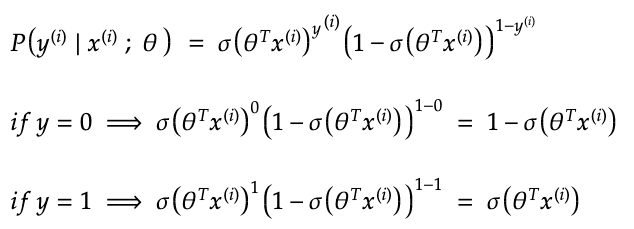
However, there is another convex cost function that can be used. The probability that an example equals 1 is:
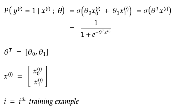
Where (i) represents a training example. The probability and example equals 0 is:
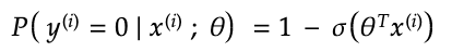
Below, is the above combined into one equation. It tells you the probability that an example falls into its true category based on the current weights. You want the answer to be close to one since it would mean that the prediction is correct.
Now, if you take the product for every example, you get the following equation:
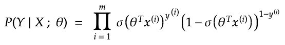
We want this number to be maximised since it would mean that the training examples are being classified correctly.
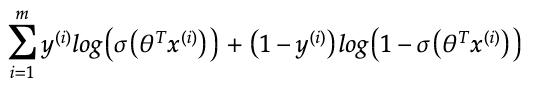
If you take the logarithm instead, you get the log likelihood which you would also want to maximize.
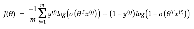
Instead, we want a cost function to minimise so we will multiply it by -1/m giving:
Below are the partial derivatives:
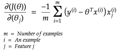
This post shows how the partial derivates of the cost function are calculated.
The video below also gives a very good explanation of how the cost function is derived. Be aware that, in the video, he does not multiply the log likelihood by -1/m which is why he says to use gradient ascent instead of descent.
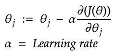
Now, to optimize the weights, you just need to go through the same process as is done with linear regression using gradient descent. So, you randomly initialize the weights, then update them using the following assignment until the weights converge to an optimum value.
What alternatives are there to logistic regression
There are many other algorithms that can be used for classification. These algorithms include decision trees, random forests, support vector machines, naive bayes, k-nearest neighbours and even neural networks. I have written about them all in this post.
Is the sigmoid function the only acceptable function?
No, other functions can be used that have a different range of possible outputs such as the tanh function which gives an output between -1 and 1. The sigmoid function is ideal if you want to get a probability estimate that an example falls into a certain class.
Neural networks used to use the sigmoid function as an activation function for every layer of the neural network. It was preferred by researchers because it is differentiable everywhere. However, it often resulted in something known as the vanishing gradient problem which was where the initial layers of a neural network would not change by much when using backpropagation. As a result, it was found that other activation functions, such as the ReLU activation function allowed the neural network to perform much better. Now, sigmoid functions are only typically used in the final output layer.
How to implement it in code
Below is an example of how to implement logistic regression using Python.
import numpy as np
import matplotlib.pyplot as plt
X = np.arange(15).reshape(-1, 1)
Y = np.array([0,0,0,0,0,0,0,1,1,1,1,1,1,1,1])
plt.scatter(X, Y)
plt.xlabel(“$x_1$”, fontsize=18)
plt.ylabel(“$y$”, rotation=0, fontsize=18)
plt.show()
from sklearn.linear_model import LogisticRegression
model = LogisticRegression().fit(X,Y)
probs = model.predict_proba(X)
probs
array([[9.99573692e-01, 4.26308310e-04],
[9.98594654e-01, 1.40534607e-03],
[9.95377606e-01, 4.62239420e-03],
[9.84907553e-01, 1.50924466e-02],
[9.51868837e-01, 4.81311630e-02],
[8.57005898e-01, 1.42994102e-01],
[6.44920520e-01, 3.55079480e-01],
[3.55014191e-01, 6.44985809e-01],
[1.42959165e-01, 8.57040835e-01],
[4.81181022e-02, 9.51881898e-01],
[1.50882090e-02, 9.84911791e-01],
[4.62108256e-03, 9.95378917e-01],
[1.40494601e-03, 9.98595054e-01],
[4.26186832e-04, 9.99573813e-01],
[1.29194486e-04, 9.99870806e-01]])
Index 0 gives the probability that an example is in the 0 category. Index 1 gives the probability that an example is in the 1 category.
plt.scatter(X, Y)
plt.plot(X, probs[:,1], color=”r”)
plt.xlabel(“$x_1$”, fontsize=18)
plt.ylabel(“$y$”, rotation=0, fontsize=18)
plt.show()
The red line represents the probability that an example equals 1.
from sklearn.metrics import confusion_matrix
confusion_matrix(Y, model.predict(X))
array([[7, 0],
[0, 8]])
The confusion matrix shows that all examples in the training set are being classified correctly.
Sources
Andrew Ng’s machine learning course on Coursera
Aurélien Géron’s Hands on machine learning with scikit-learn and tensorflow
https://scikit-learn.org
Elements of Statistical Learning http://faculty.marshall.usc.edu/gareth-james/ISL/
https://www.youtube.com/watch?v=TM1lijyQnaI