
Multiple linear regression is one of the key algorithms used in machine learning. This post will show you how it works and how to implement it, in code, using Python.
This post is a continuation of linear regression explained, if you are not familiar with linear regression for a single feature variable, please read it then come back to this post.
The basics of multiple linear regression
The goal of linear regression with a single variable is to fit a line to the data. The goal of multiple linear regression is to fit a hyperplane to data so that we can make predictions using multiple feature variables.
When to use it
Multiple linear regression can be used when the independent variables (the factors you are using to predict with) each have a linear relationship with the output variable (what you want to predict).
So, the equation between the independent variables (the X values) and the output variable (the Y value) is of the form Y= θ0+θ1X1+θ2X2+…+θnXn (linear) and it is not of the form Y=θ0+θ1e^X1+… or Y = θ0+θ1X1X2+… (non-linear).
Below are some possible examples where multiple linear regression might be appropriate:
- Predicting the price of a house based on the median income in the area and the number of rooms in the house.
- Predicting the number of ice cream sales based on the price and the temperature.
How it works
With linear regression for a single variable, our goal was to find optimum values for θ0 and θ1 in the equation Y=θ0+θ1X1 that allow us to fit the best possible line through the data. With multiple linear regression, our goal is to find optimum values for θ0, θ1,…,θn in the equation
Y= θ0+θ1X1+θ2X2+…+θnXn
where n is the number of different feature variables.
The process of optimizing the weights is identical to the process for linear regression with a single variable. Except, now we just have some more features to deal with.
Term definitions:
m = The number of examples in the dataset
n = The number of features in the dataset
xi1 = The x value of the ith training example of the first feature
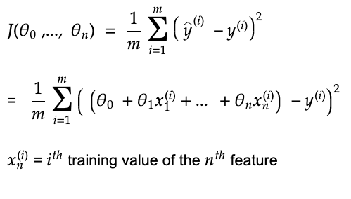
yhat = The prediction of the true Y value for a training example = θ0+θ1xi1+…+θnxin
θ0 = the y-intercept (also known as the bias)
θn = The coefficient being used to multiply Xn (also known as the weight)
This is the process of how to optimize the weights
1 Set θ0=0, θ1=0, …, θn=0
2. Define a cost function
As before, we need a way to measure how well our current weights are performing. Again, to do this, we will take the sum of the squared differences between our predictions using our current yhat and the actual y values.
3 Use the cost function to optimize the values of θ0=0, θ1=0, …, θn=0
As before, we will use gradient descent to optimize the values of θ0=0, θ1=0, …, θn=0
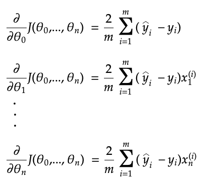
The partial derivates are:
Below is the gradient descent algorithm for multiple linear regression:
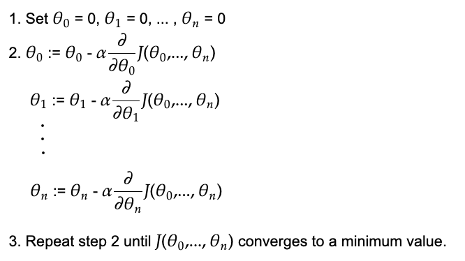
:= means to assign a new value.
α (Alpha) is called the learning rate which controls how quickly to converge to the optimum values for θ0, θ1, …, θn.
The partial derivatives of J(θ0, …,θn) with respect to θ0, θ1,…,θn tells us the slope of the function at the current values of θ0, θ1,…,θn. Gradient descent then uses the partial derivatives to update the values of θ0, θ1,…,θn by subtracting the value of the partial derivative, multiplied by the learning rate, from the current values.
Each time, we update the values of θ0, θ1,…θn, using their partial derivatives, we get closer to their optimum values. Each time we get closer, the slope of the partial derivatives will reduce. This is a good thing since the closer we get to the optimum values of θ0, θ1,…,θn, the smaller we want each change of their values to be.
The reason why the learning rate is necessary is that it is possible to increase or decrease θ0, θ1,…,θn by too much causing them to diverge away from the optimum values. A traditional default value for the learning rate is 0.1 or 0.01.
If you are having an issue with the learning rate, it would help to find a high learning rate where the cost actually diverges and a very low learning rate that does approach an optimum value but too slowly. Then it should become easier to find an optimal learning rate in between that converges towards an optimal value reasonably quickly.
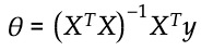
Analytical solution
There is an equation that allows you to calculate each of the weights directly as shown below. However, the computational complexity is up to O(n^3) depending on the implementation.
Is it necessary to scale the features?
When you are using gradient descent, you should scale the features. This is because it helps gradient descent to converge faster. The reason for this is that it allows gradient descent to take a more direct path towards the global minimum because the learning rate is the same for each weight. This means that the size of the step on each gradient descent step might be too steep for some weights and not steep enough for others. However, this is not such an issue for more recent optimizer algorithms that compute the learning rate for each feature on each descent step as shown here.
One way to scale the features is to divide each feature value by the range of that feature’s values.
The video below shows you why feature scaling helps with regular gradient descent.
Is it necessary to get rid of outliers?
Outliers can significantly affect the weights in the model. However, it is not always a good idea to remove them. Sometimes, outliers are there because of data entry errors or because they do not belong to the population you’re studying and they should be removed.
However, sometimes, the outliers are there due to legitimate causes, and removing them could cause your model to be less reliable. You can read more about determining whether or not to remove outliers here. I also found this Udemy course to be quite comprehensive when it comes to feature engineering and it talks about dealing with outliers.
Code example
Here is how to implement multiple linear regression, in Python, using sklearn:
import numpy as np
from sklearn import datasets
from sklearn.linear_model import LinearRegression
from sklearn.model_selection import train_test_split
from sklearn.metrics import mean_squared_error, r2_score
X, y = datasets.load_diabetes(return_X_y=True)
X_train,X_test,y_train,y_test = train_test_split(X,y,test_size=0.2)
reg = LinearRegression().fit(X_train, y_train)
reg.intercept_, reg.coef_
(151.06925805841755, array([ 54.52885236, -287.65356694, 546.96003617, 337.11892523, -749.7977235 , 403.8751115 , 109.85313395, 218.18005015, 722.75246222, 64.94051697]))
This represents the equation:
Y_hat = 151+54*X1 – 287*X2 + 546*X3 + 337*X4 – 749*X5 + 403*X6 + 109*X7 + 218*X8 + 722*X9 + 64*x10
preds = reg.predict(X_test)
print(‘Mean squared error: %.2f’ % mean_squared_error(y_test, preds))
print(‘Coefficient of determination: %.2f’ % r2_score(y_test, preds))
Mean squared error: 2899.82 Coefficient of determination: 0.43
Sources
Andrew Ng’s machine learning course on Coursera
Aurélien Géron’s Hands on machine learning with scikit-learn and tensorflow
https://scikit-learn.org