
Linear regression is one of the key algorithms used in machine learning. In this post, I will show you what linear regression is, then I will show you how to implement it in code using Python.
The basics of linear regression
The goal of linear regression is to fit a line to data so that we can make predictions using the equation of that line.
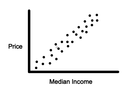
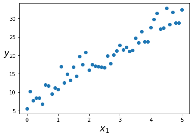
So, if we have data, such as in the image below…
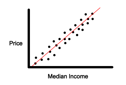
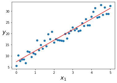
Linear regression will allow us to find a line such as the one in the image below that allows us to make predictions on new data points.
When to use linear regression
Linear regression can be used when the independent variable (the factor you are using to predict with) has a linear relationship with the output variable (what you want to predict).
So, the equation between the independent variable (the X value) and the output variable (the Y value) is of the form Y= θ0+θ1X1 (linear) and it is not of the form Y=θ0+θ1e^X1 or Y = θ0+θ1X1X2 (non-linear).
Examples could be predicting the price of a house based on the median income in the area, the number of expected sales on a particular day based on the temperature, or the number of tickets that will be sold based on the price.
How linear regression works
Our goal is to find optimum values for θ0 and θ1 in the equation Y=θ0+θ1X1 that allow us to fit the best possible line through the data. This is so that we can make the most accurate predictions possible.
Here is an example dataset that we will use below:
| X | Y |
| 1 | 1 |
| 2 | 3 |
| 3 | 3 |
| 4 | 4 |
| 5 | 6 |
Term definitions:
m = The number of examples in the dataset (5 in the example above)
xi = The x value of the ith training example (ie x2 = 2 in the example above)
yhat = The prediction of the true Y value for a training example = θ0+θ1xi
θ0 = the y-intercept (also known as the bias)
θ1 = The coefficient being used to multiply X1 (also known as the weight)
This is the process of how we will do it:
- We will initially set θ0=0 and θ1=0 so that Yhat = 0+0X1
- We will define a cost function that will allow us to measure how bad the Yhat currently is.
- We will then iterate through each training example and use them to update the current values of θ0 and θ1 using an algorithm called gradient descent.
- Set θ0=0 and θ1=0
First, we set θ0=0 and θ1=0. Other algorithms, in machine learning, start by initializing the weights randomly. However, the cost function we will be using is convex which means that the initial weights are not so important.
2. Define a cost function
We need a way to measure how well our current θ0 and θ1 values are performing so that we can figure out how to improve them.
To do this, we will take the sum of the squared differences between our predictions using our current yhat and the actual y values.
This is done with the following equation:
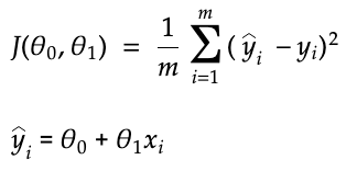
The above equation is known as the “mean squared error cost function” (MSE).
Visually, we are taking the sum of the vertical lines in the image below. The reason why we are squaring the distances is to avoid having negative values canceling out positive values. The vertical lines are equal to the difference between our predicted value of an example and the actual value.

3. Use the cost function to optimize the values of θ0 and θ1
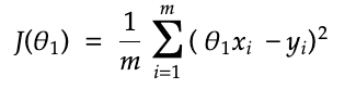
If we temporarily ignore θ0 and imagine that we only have to worry about optimizing θ1, we would have the equation yhat = θ1X1. So, the cost function would become:
Different values of θ1 will result in a different value for the cost function J(θ1). If we were to plot these values on a graph we would end up with one that looks like the graph below:

Where the graph is at its minimum, θ1 is at its optimum value. The derivative of a function tells us the slope of a curve at a point. This means that when the derivative of J(θ1) = 0
θ1 is at its optimum value.
If we now reconsider the case where we include the bias term θ0, it is also the case that J(θ0,θ1) has optimum values for θ0 and θ1. However, in this case, it will be necessary for us to minimize the partial derivative of J(θ0,θ1) with respect to θ0 and the partial derivative with respect to θ1.
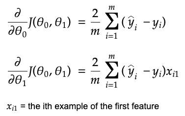
Below are the partial derivates with respect to both θ0 and θ1:
Now that we know what the partial derivatives are we can now devise an algorithm that will allow us to come to the optimal values for θ0 and θ1. The algorithm we will use is called “gradient descent”. The image below describes how it works:
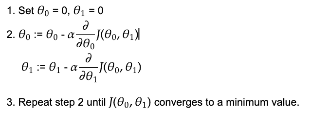
:= means to assign a new value.
α (Alpha) is called the learning rate which controls how quickly to converge to the optimum values for θ0 and θ1.
The partial derivatives of J(θ0, θ1) with respect to θ0 and θ1 tells us the slope of the function at the current values of θ0 and θ1. Gradient descent then uses the partial derivatives to update the values of θ0 and θ1 by subtracting the value of the partial derivative, multiplied by the learning rate, from the current values.
Each time, we update the values of θ0 and θ1, using their partial derivatives, we get closer to their optimum values. Each time we get closer, the slope of the partial derivatives will reduce. This is a good thing since the closer we get to the optimum values of θ0 and θ1, the smaller we want each change of their values to be.
The reason why the learning rate is necessary is that it is possible to increase or decrease θ0 and θ1 by too much causing them to diverge away from the optimum values. A traditional default value for the learning rate is 0.1 or 0.01.
What output does linear regression give?
Linear regression gives a continuous output that can be greater than 1, less than 0 or any number in between. This means that it does not give you the probability of a particular outcome. However, it can be used to predict things that have infinite possible answers.
Alternatives to gradient descent
Gradient descent is not the only option for finding the optimal weight values for linear regression. However, in the context of machine learning, it is the most commonly used algorithm and it is used to optimize other machine learning algorithms as well.
Another algorithm for optimizing linear regression, often used in statistics, is ordinary least squares.
There is also a closed-form solution allowing you to calculate the weights with matrix operations. The issue with it is that it has an algorithmic complexity of O(n^3). You can read more about it here.
How to implement Linear Regression in code
Here is how to implement linear regression, in Python, using sklearn:
import numpy as np
import matplotlib.pyplot as plt
X_values = np.arange(0,5.1,0.1).reshape(-1,1)
Y_values = 4 + 5 * X_values + 8*np.random.rand(51,1)
plt.scatter(X_values, Y_values)
plt.xlabel(“$x_1$”, fontsize=18)
plt.ylabel(“$y$”, rotation=0, fontsize=18)
plt.show()
from sklearn.linear_model import LinearRegression
reg = LinearRegression().fit(X_values, Y_values)
reg.intercept_, reg.coef_
(array([7.37957952]), array([[4.78145655]]))
This represents the equation Y_hat = 7.379 + 4.78*X
plt.scatter(X_values, Y_values)
plt.plot(X_values, reg.predict(X_values), color=”r”)
plt.xlabel(“$x_1$”, fontsize=18)
plt.ylabel(“$y$”, rotation=0, fontsize=18)
plt.show()
Sources
Andrew Ng’s machine learning course on Coursera
Aurélien Géron’s Hands on machine learning with scikit-learn and tensorflow
The Scikit-learn docs https://scikit-learn.org